Electric and Magnetic Fields

Point Charge

A point charge is a point particle with nonzero electric charge and infinitesimal volume.

Coulombs Law

Also called Coulomb's inverse-square law states the magnitude of the attraction or repulsion electrostatic force ($\bm{F}$) between two charges is directly proportional to the magnitude of charges ($q$) and inversely proportional to the square of the magnitude of the separation displacement ($\bm{r}$):

\begin`\{aligned}` |\bm{F}| \propto |q_1||q_2|, \quad |\bm{F}| \propto |\bm{r}|^2\\ |\bm{F}| = k \frac{|q_1||q_2|}{|\bm{r}|^2} \end`\{aligned}`

info

Coulomb's Law can also be expressed in vector form, where the force exerted by $q_1$ on $q_2$ is:

\begin`\{aligned}` \bm{F_{12}} = k \frac{q_1 q_2}{|r|^2} \hat{r_{12}} = -\bm{F_{21}} \end`\{aligned}`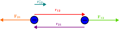

Where the constant $k$ is named Coulomb's constant and is equal to:

\begin`\{aligned}` k = \frac{1}{4\pi \epsilon_0} \end`\{aligned}`

info

The derivation of Coulomb's constant can be possible with Maxwell's equations. Gauss's Law states that the electric flux ($\Phi$) through any closed surface is equal to net electric charge enclosed within the surface multiply by the inverse of permittivity of free space ($\epsilon_0$):

\begin`\{aligned}` \Phi = \oiint\limits_{S} E \cdot dA = \frac{Q}{\epsilon_0} \end`\{aligned}`

For a point charge, symmetry implies a radial electric field, and hence a sphere enclosed surface ($4\pi r^2$), therefore, simplifying $\phi$ to:

\begin`\{aligned}` \Phi = 4\pi r^2 = \frac{Q}{\epsilon_0}\\ E = \left(\frac{1}{4\pi\epsilon_0}\right)\left(\frac{Q}{r^2}\right)\\ F = q_2 E = \frac{1}{4\pi \epsilon_0} \frac{|q_1||q_2|}{r^2} \end`\{aligned}`

Coulomb's constant can now be identify as:

\begin`\{aligned}` k = \frac{1}{4\pi \epsilon_0} \end`\{aligned}`

Electric Field

Charges and Fields

Place positive and negative charges on the canvas and observe the resulting electric field lines and equipotential surfaces. Drag a test charge to feel the force at different positions.

The electric field $\bm{E}$ with vector quantity of electrostatic force $\bm{F}$ exerted per unit of magnitude of charge, evaluated as:

\begin`\{aligned}` \bm{E} = \lim_{q \rightarrow 0} \frac{F}{q} \end`\{aligned}`

Electric Potential Energy

Electric potential energy ($U$ or $E_p$ or $W$)is the minimum work required to translate charges from infinite separation displacement to a position $\bm{r}$. Since the electrostatic force $\bm{F_e}$ varies due to the displacement, the line integral of the opposing force $\bm{F_{ext}} = \bm{F_e}$ from infinity $(\infty)$ to the potion $\bm{r}$ gives the work required to translate the charges:

\begin`\{aligned}` U &= E_p = W = \int_\infty^{\bm{r}} F_`\{ext}` \cdot d\bm{r} = -\int_\infty^{\bm{r}} F_e \cdot \bm`\{dr}`\\ U &= -\int_\infty^{\bm{r}} \left(k\frac{q_1 q_2}{|\bm{r}|^2}\bm{\hat{r}}\right) \cdot \bm`\{dr}` \end`\{aligned}`

Separating the magnitude and direction of $\bm{dr}$ gives $d|\bm{r}|\bm{\hat{r}}$, and hence changing the bounds ($\bm{r} \rightarrow |\bm{r}|$):

\begin`\{aligned}` U &= -\int_\infty^{|\bm{r}|} \left(k\frac{q_1 q_2}{|\bm{r}|^2}\bm{\hat{r}}\right) \cdot d|\bm{r}|\bm{\hat{r}}\\ U &= -\frac{q_1 q_2}{4\pi\epsilon_0} \int_\infty^{|\bm{r}|} \frac{1}{|\bm{r}|^2} d|\bm{r}|\\ U &= -\frac{q_1 q_2}{4\pi\epsilon_0} \left[-\frac{1}{|\bm{r}|}\right]_\infty^{|\bm{r}|}\\ U &= \frac{1}{4\pi \epsilon_0}\frac{q_1 q_2}{|\bm{r}|} \end`\{aligned}`

This is written in the formula booklet with $r = |\bm{r}|$ and Coulomb's constant $k$:

\begin`\{aligned}` U = k\frac{q_1 q_2}{r} \end`\{aligned}`

This implies the electric potential energy is a scalar quantity approaching $0$ at infinite displacement $r \rightarrow \infty$.

Electric Potential

The electric potential ($V_e$) is the electric potential energy of a point charge ($Q$ or $q_1$) at displacement $\bm{r}$ per unit charge:

\begin`\{aligned}` V_e &= \frac{U}{q_2} = \frac{1}{4\pi \epsilon_0}\frac{q_1 q_2}{|\bm{r}|q_2} = \frac{1}{4\pi \epsilon_0}\frac{Q}{|\bm{r}|}\\ V_e &= \frac`\{kQ}`{r}, \quad r = |\bm{r}| \end`\{aligned}`

Electric Field Strength

The electric field strength ($\bm{E}$) is the force ($\bm{F_{12}}$) per unit charge of the affected point charge ($q_2$) at a displacement ($\bm{r_{12}}$):

\begin`\{aligned}` \bm{E} = \frac{\bm{F_{12}}}{q_2} = \frac{1}{4\pi \epsilon_0} \frac{q_1 q_2}{|\bm{r}|^2}\bm{\hat{r_{12}}} \end`\{aligned}`

This is written in the formula booklet with $d = |\bm{r}|$:

\begin`\{aligned}` E = \frac{F}{q} = k\frac{Q}{d^2} \end`\{aligned}`

The electric field strength is also the negative gradient of the electric potential ($V_e$):

\begin`\{aligned}` E = -\nabla V_e \end`\{aligned}`

Since spherical symmetry implies the gradient of electric potential are equal for equal magnitude of displacement $\bm{r}$:

\nabla V_e = \frac{dV_e}{d|\bm{r}|}\bm{\hat{r}}\\ \frac{dV_e}{d|\bm{r}|} = \frac{d}{d|\bm{r}|}\left(\frac`\{kQ}`{|\bm{r}|}\right) = -k\frac{Q}{|\bm{r}|^2}\\ E = k \frac{Q}{|\bm{r}|^2}\bm{\hat{r}}

When expressing the electric field strength with the average electric potential change, and expressing $r = |\bm{r}|$, the magnitude of $E$ is:

\begin`\{aligned}` E = -\frac{\Delta V_e}{\Delta r} \end`\{aligned}`

Graphical Presentation of Electric Field

Electric Field Lines

Electric field lines present the direction of electric field strength.

Equipotential Surfaces

Equipotential surfaces are surfaces with equivalent electric potential.

Millikan's Experiment

The Millikan's experiment was conducted in 1909 to determine the value of elementary charge. The experiment was passing ionized oil drops with charge $q$ within a region between two charged metal plates with a electric potential $V_e$, and displacement $\bm{d}$. The IB include a simplified calculation for elementary charge by ignoring buoyance force, where the electrostatic force ($\bm{F_e}$) equal to the opposite of gravitational force ($\bm{F_g}$):

\begin`\{aligned}` \bm{F_g} &= -\bm{F_e}\\ \bm{F_g} &= m\bm{g}\\ -\bm{F_e} &= -qE = -q\left(-\frac{V_e}{\bm{d}}\right)\\ m\bm{g} &= q\frac{V_e}{\bm{d}}\\ q &= \frac{m\bm{g}\bm{d}}{V_e} \end`\{aligned}`

---

Electric Field Between Parallel Plates

When two parallel conducting plates are separated by a distance $d$ and a potential difference $V$ is applied across them, a uniform electric field is created between the plates:

$$E = \frac{V}{d}$$

Key properties:

• The field is uniform (constant magnitude and direction) between the plates.
• The field lines are parallel and equally spaced.
• Fringing occurs at the edges of the plates (the field is not perfectly uniform there, but this is usually neglected in IB problems).

Worked Example: Parallel Plates

Question: Two parallel plates are separated by 2.0 cm with a potential difference of 500 V. An electron is placed midway between the plates. What is the force on the electron and the acceleration?

Solution:

$$E = \frac{V}{d} = \frac{500}{0.020} = 2.5 \times 10^4 \mathrm{ V/m}$$ $$F = eE = (1.60 \times 10^{-19})(2.5 \times 10^4) = 4.0 \times 10^{-15} \mathrm{ N}$$ $$a = \frac{F}{m_e} = \frac{4.0 \times 10^{-15}}{9.11 \times 10^{-31}} = 4.39 \times 10^{15} \mathrm{ m/s}^2$$

Exam tip: Remember that the force on an electron is directed from the negative plate toward the positive plate (opposite to the field direction, since the electron has negative charge).

---

Electric Field Strength Due to a Point Charge

The electric field strength at a distance $r$ from a point charge $Q$ is:

E = \frac`\{kQ}`{r^2} = \frac{Q}{4\pi\epsilon_0 r^2}

Direction: Radially outward from a positive charge, radially inward toward a negative charge.

Superposition of Electric Fields

When multiple charges are present, the total electric field at any point is the vector sum of the individual fields:

$$\bm{E}_{\mathrm{total}} = \bm{E}_1 + \bm{E}_2 + \bm{E}_3 + \cdots$$

Worked Example: Superposition

Question: Two point charges, $q_1 = +3.0 \mathrm{ \mu C}$ and $q_2 = -5.0 \mathrm{ \mu C}$, are placed 20 cm apart. Find the electric field strength at the midpoint between them.

Solution:

Distance from each charge to midpoint: $r = 0.10$ m.

$$E_1 = \frac{kq_1}{r^2} = \frac{(8.99 \times 10^9)(3.0 \times 10^{-6})}{(0.10)^2} = 2.70 \times 10^6 \mathrm{ V/m} \quad \mathrm{(away from } q_1)$$ $$E_2 = \frac{k|q_2|}{r^2} = \frac{(8.99 \times 10^9)(5.0 \times 10^{-6})}{(0.10)^2} = 4.50 \times 10^6 \mathrm{ V/m} \quad \mathrm{(toward } q_2)$$

Since both fields point in the same direction at the midpoint (from $q_1$ toward $q_2$):

$$E_{\mathrm{total}} = E_1 + E_2 = 2.70 \times 10^6 + 4.50 \times 10^6 = 7.20 \times 10^6 \mathrm{ V/m}$$

---

Electric Potential

The electric potential ($V_e$) at a point is the electric potential energy per unit charge at that point. It is a scalar quantity.

For a point charge $Q$:

V_e = \frac`\{kQ}`{r}

Key properties:

• $V_e$ is positive near positive charges and negative near negative charges.
• $V_e = 0$ at infinity (by convention).
• The electric field strength is the negative gradient of the potential: $E = -\frac{\Delta V_e}{\Delta r}$.

Equipotential Surfaces

Equipotential surfaces are surfaces of constant electric potential. Key properties:

• Electric field lines are always perpendicular to equipotential surfaces.
• No work is done moving a charge along an equipotential surface.
• For a point charge, equipotential surfaces are concentric spheres.
• For parallel plates, equipotential surfaces are parallel planes.

---

Capacitors

A capacitor is a device that stores electric charge and energy. The simplest form consists of two parallel conducting plates separated by an insulator (dielectric).

Capacitance

Capacitance ($C$) is defined as the charge stored per unit potential difference:

$$C = \frac{Q}{V}$$

The unit of capacitance is the farad (F). Typical capacitor values range from picofarads (pF) to millifarads (mF).

Capacitance of a Parallel Plate Capacitor

$$C = \frac{\epsilon_0 A}{d}$$

where:

• $\epsilon_0 = 8.85 \times 10^{-12}$ F/m is the permittivity of free space
• $A$ is the area of one plate (m²)
• $d$ is the separation between plates (m)

Energy Stored in a Capacitor

$$W = \frac{1}{2}QV = \frac{1}{2}CV^2 = \frac{Q^2}{2C}$$

These three expressions are equivalent (using $Q = CV$). Use whichever is most convenient given the known quantities.

Worked Example: Capacitor Energy

Question: A 100 $\mu$F capacitor is charged to a potential difference of 200 V. How much energy does it store?

Solution:

$$W = \frac{1}{2}CV^2 = \frac{1}{2}(100 \times 10^{-6})(200)^2 = \frac{1}{2}(100 \times 10^{-6})(40000) = 2.0 \mathrm{ J}$$

---

Magnetic Fields

Sources of Magnetic Fields

• Permanent magnets: Produce a magnetic field due to the alignment of magnetic domains.
• Current-carrying conductors: A current produces a magnetic field around it (Ampere's law).
• Earth: The Earth has a magnetic field, approximately that of a dipole, with the geographic south pole near the magnetic north pole.

Magnetic Field Lines

Magnetic field lines represent the direction of the magnetic field:

• They point from north to south outside a magnet.
• They form closed loops (they always form continuous loops, unlike electric field lines).
• The density of field lines indicates the strength of the field.
• Field lines never cross.

Magnetic Field of a Long Straight Wire

The magnetic field at a distance $r$ from a long straight wire carrying current $I$ is:

$$B = \frac{\mu_0 I}{2\pi r}$$

where $\mu_0 = 4\pi \times 10^{-7}$ Tm/A is the permeability of free space.

The direction is given by the right-hand grip rule: grip the wire with your right hand, thumb pointing in the direction of conventional current, and your fingers curl in the direction of the magnetic field.

Magnetic Field Inside a Solenoid

A solenoid is a long coil of wire. Inside an ideal solenoid:

$$B = \mu_0 n I$$

where $n$ is the number of turns per unit length ($n = N/L$).

The field inside a solenoid is approximately uniform and parallel to the axis. The field outside is approximately zero.

---

Comparison: Electric vs Magnetic Fields

Property	Electric Field	Magnetic Field
Source	Stationary or moving charges	Moving charges (currents)
Force on charge	$F = qE$ (parallel to E)	$F = qvB\sin\theta$ (perpendicular to v and B)
Does work on charge	Yes	No (always perpendicular to velocity)
Field lines	Start on + charges, end on - charges	Form closed loops (no monopoles)
Units	V/m or N/C	Tesla (T)
Constant	$\epsilon_0$ (permittivity)	$\mu_0$ (permeability)

---

Exam Tips for D.2 (Electric and Magnetic Fields)

1. Coulomb's law vs gravitational force: Both are inverse-square laws, but electric forces can be attractive or repulsive, while gravitational forces are always attractive.

2. Sign conventions for electric potential: The electric potential energy of two like charges is positive (repulsive); for two unlike charges, it is negative (attractive). The potential energy is zero at infinite separation.

3. Distinguish between electric potential ($V_e$) and electric field strength ($E$): Potential is a scalar; field strength is a vector. They are related by $E = -\Delta V_e / \Delta r$.

4. For parallel plate problems: Always identify whether you need $E = V/d$ or $E = \sigma / \epsilon_0$ (the latter is beyond IB scope but good to know). The IB formula is $E = V/d$.

5. Millikan's experiment: Be able to explain how balancing gravitational and electric forces on a charged oil drop allows the determination of the elementary charge. The key equation is $q = mgd/V$.

6. Capacitors: Remember that capacitance depends only on the geometry of the plates ($A$, $d$) and the dielectric, not on the charge or voltage. The energy stored can be expressed in three equivalent forms — use the one that matches your given data.

7. Unit conversions: Electric fields are often in V/m or N/C (equivalent). Capacitance is in farads (F), but practical values are in $\mu$F, nF, or pF. Be comfortable converting between SI prefixes.

---

Worked Example: Magnetic Force on a Current-Carrying Wire

Problem: A straight wire of length 0.50 m carrying a current of 3.0 A is placed in a uniform magnetic field of $B = 0.40$ T. The wire makes an angle of $60^\circ$ with the field. Calculate the magnitude of the force on the wire.

Solution:

$$F = BIL\sin\theta = (0.40)(3.0)(0.50)\sin 60^{\circ} = (0.60)(0.866) = 0.520 \mathrm{ N}$$

The direction is given by Fleming's Left-Hand Rule: first finger along $\bm{B}$, second finger along $I$, thumb gives the direction of $\bm{F}$.

---

Worked Example: Parallel Plate Capacitor Design

Problem: A parallel plate capacitor is to be designed with a capacitance of $100$ pF using plates of area $0.010$ m$^2$. a) What plate separation is required? b) If the capacitor is charged to 200 V, how much charge is stored? c) What is the energy stored?

Solution:

a) Plate separation:

$$C = \frac{\epsilon_0 A}{d} \implies d = \frac{\epsilon_0 A}{C} = \frac{(8.85 \times 10^{-12})(0.010)}{100 \times 10^{-12}} = \frac{8.85 \times 10^{-14}}{10^{-10}} = 8.85 \times 10^{-4} \mathrm{ m} = 0.885 \mathrm{ mm}$$

b) Charge stored:

$$Q = CV = (100 \times 10^{-12})(200) = 2.0 \times 10^{-8} \mathrm{ C} = 20 \mathrm{ nC}$$

c) Energy stored:

$$W = \frac{1}{2}CV^2 = \frac{1}{2}(100 \times 10^{-12})(200)^2 = \frac{1}{2}(100 \times 10^{-12})(40000) = 2.0 \times 10^{-6} \mathrm{ J} = 2.0 \mathrm{ \mu J}$$

---

Worked Example: Electric Field Lines and Equipotentials

Problem: A positive point charge $Q = +5.0$ nC is placed at the origin. a) Calculate the electric field strength at a point 0.10 m from the charge along the x-axis. b) Calculate the electric potential at that point. c) A second charge $q = -2.0$ nC is placed at that point. What is the electric potential energy of the system?

Solution:

a) Electric field strength:

E = \frac`\{kQ}`{r^2} = \frac{(8.99 \times 10^9)(5.0 \times 10^{-9})}{(0.10)^2} = \frac{44.95}{0.01} = 4.50 \times 10^3 \mathrm{ V/m}

Direction: radially outward from $Q$ (away from the positive charge).

b) Electric potential:

V_e = \frac`\{kQ}`{r} = \frac{(8.99 \times 10^9)(5.0 \times 10^{-9})}{0.10} = \frac{44.95}{0.10} = 450 \mathrm{ V}

c) Electric potential energy:

$$U = qV_e = (-2.0 \times 10^{-9})(450) = -9.0 \times 10^{-7} \mathrm{ J} = -900 \mathrm{ nJ}$$

The negative sign indicates the system is bound (attractive), which is expected for opposite charges.

---

Gauss's Law (Qualitative Treatment)

Gauss's Law provides a powerful way to calculate electric fields for symmetric charge distributions. It states:

$$\Phi_E = \oiint_S \bm{E} \cdot d\bm{A} = \frac{Q_{\mathrm{enclosed}}}{\epsilon_0}$$

where $\Phi_E$ is the electric flux through a closed surface $S$, and $Q_{\mathrm{enclosed}}$ is the total charge inside that surface.

Key implications:

• The electric flux through a closed surface depends only on the enclosed charge, not on the distribution of charge outside the surface.
• For a point charge, choosing a spherical Gaussian surface gives $E = \frac{Q}{4\pi\epsilon_0 r^2}$.
• For a charged conducting sphere, the electric field outside is the same as a point charge at the center, and the field inside the conductor is zero (charges reside on the surface).
• Between parallel plates, using a rectangular Gaussian surface shows that the field is uniform: $E = \frac{\sigma}{\epsilon_0}$ where $\sigma$ is the surface charge density.

Exam tip: For the IB, you need to understand Gauss's Law qualitatively. Be able to explain why the field inside a conductor is zero, and why the field outside a charged sphere behaves like a point charge.

---

Common Pitfalls

1. Forgetting that electric potential is a scalar. When calculating the total potential at a point due to multiple charges, add the potentials algebraically (including signs). Do not use vector addition.

2. Confusing electric potential energy and electric potential. Potential energy $U$ depends on both charges ($U = kq_1 q_2 / r$). Potential $V_e$ is the energy per unit charge ($V_e = kQ / r$).

3. Using the wrong formula for the force between charges. Coulomb's law gives the force between point charges. For parallel plates, use $F = qE$ where $E = V/d$.

4. Ignoring the sign of the charge in electric field direction. The electric field points away from positive charges and toward negative charges. The force on a positive charge is in the direction of $\bm{E}$; the force on a negative charge is opposite to $\bm{E}$.

5. Capacitance is a property of the geometry, not the charge or voltage. Changing the charge on a capacitor does not change its capacitance. $C = \epsilon_0 A / d$ depends only on plate area and separation.

6. Magnetic force direction errors. For a current-carrying wire, use Fleming's Left-Hand Rule. For a moving charge, use the right-hand rule (and reverse for negative charges).

---

Problem Set

Question 1

Two point charges $q_1 = +4.0$ $\mu$C and $q_2 = -6.0$ $\mu$C are placed 30 cm apart in vacuum. a) Calculate the electric force between them. b) Is the force attractive or repulsive? Justify your answer.

Answer 1

a) $F = \frac{k|q_1||q_2|}{r^2} = \frac{(8.99 \times 10^9)(4.0 \times 10^{-6})(6.0 \times 10^{-6})}{(0.30)^2} = \frac{215.8}{0.09} = 2.40 \times 10^3$ N $= 2.40$ kN.

b) The force is attractive because the charges have opposite signs (one positive, one negative). Coulomb's law gives a negative value for the product $q_1 q_2$, indicating attraction.

Question 2

A parallel plate capacitor has plates of area $200$ cm$^2$ separated by $2.0$ mm. A potential difference of 500 V is applied. Calculate: a) The capacitance. b) The charge on each plate. c) The electric field strength between the plates. d) The energy stored.

Answer 2

a) $C = \frac{\epsilon_0 A}{d} = \frac{(8.85 \times 10^{-12})(200 \times 10^{-4})}{2.0 \times 10^{-3}} = \frac{1.77 \times 10^{-13}}{2.0 \times 10^{-3}} = 8.85 \times 10^{-11}$ F $= 88.5$ pF.

b) $Q = CV = (8.85 \times 10^{-11})(500) = 4.43 \times 10^{-8}$ C $= 44.3$ nC.

c) $E = \frac{V}{d} = \frac{500}{2.0 \times 10^{-3}} = 2.5 \times 10^5$ V/m.

d) $W = \frac{1}{2}CV^2 = \frac{1}{2}(8.85 \times 10^{-11})(500)^2 = \frac{1}{2}(8.85 \times 10^{-11})(250000) = 1.11 \times 10^{-5}$ J $= 11.1$ $\mu$J.

Question 3

An electron is accelerated from rest through a potential difference of 1000 V. Calculate: a) The kinetic energy gained by the electron in electron-volts. b) The speed of the electron.

Answer 3

a) The kinetic energy gained equals the work done by the electric field: $E_k = qV = eV = 1000$ eV $= 1.60 \times 10^{-16}$ J.

b) $E_k = \frac{1}{2}m_e v^2 \implies v = \sqrt{\frac{2E_k}{m_e}} = \sqrt{\frac{2(1.60 \times 10^{-16})}{9.11 \times 10^{-31}}} = \sqrt{3.51 \times 10^{14}} = 1.88 \times 10^7$ m/s.

Question 4

A wire of length 0.30 m carries a current of 5.0 A perpendicular to a uniform magnetic field of $B = 0.60$ T. Calculate: a) The magnetic force on the wire. b) The minimum mass that this force could support against gravity ($g = 9.8$ m/s$^2$).

Answer 4

a) $F = BIL\sin 90^{\circ} = (0.60)(5.0)(0.30)(1) = 0.90$ N.

b) For the force to support a mass against gravity: $F = mg \implies m = \frac{F}{g} = \frac{0.90}{9.8} = 0.0918$ kg $= 91.8$ g.

Question 5

Two identical positive charges of $+2.0$ $\mu$C are placed on the x-axis at $x = -0.10$ m and $x = +0.10$ m. Calculate the electric field strength at the origin. Explain why the field at the origin is zero.

Answer 5

At the origin, the distance to each charge is $r = 0.10$ m.

$E_1 = \frac{kq}{r^2} = \frac{(8.99 \times 10^9)(2.0 \times 10^{-6})}{(0.10)^2} = 1.80 \times 10^6$ V/m (directed toward the negative x-direction, away from the charge at $x = +0.10$).

$E_2 = \frac{kq}{r^2} = 1.80 \times 10^6$ V/m (directed toward the positive x-direction, away from the charge at $x = -0.10$).

The total field is: $\bm{E}_{\mathrm{total}} = \bm{E}_1 + \bm{E}_2 = -1.80 \times 10^6 + 1.80 \times 10^6 = 0$ V/m.

The field is zero because the charges are equidistant from the origin, have equal magnitude, and the fields they produce point in exactly opposite directions, cancelling completely. This point is between the charges and is a point of zero field (but not zero potential).

Question 6

Explain why the electric field inside a charged conductor is zero, making reference to Gauss's Law.

Answer 6

Inside a conductor in electrostatic equilibrium, all excess charge resides on the surface. Consider a Gaussian surface placed entirely inside the conductor. Since there is no charge enclosed by this surface ($Q_{\mathrm{enclosed}} = 0$), Gauss's Law gives:

$\Phi_E = \frac{Q_{\mathrm{enclosed}}}{\epsilon_0} = 0$

This means the net electric flux through the Gaussian surface is zero. The only way this can be true for an arbitrary Gaussian surface inside the conductor is if the electric field is zero everywhere inside. If there were a non-zero field, free electrons in the conductor would move in response, redistributing charge until the field becomes zero. This is the condition of electrostatic equilibrium.

---

Related Content at Other Levels

• A-Level Fields: Physics

---

tip

Diagnostic Test Ready to test your understanding of Electric and Magnetic Fields? The diagnostic test contains the hardest questions within the IB specification for this topic, each with a full worked solution.

Unit tests probe edge cases and common misconceptions. Integration tests combine Electric and Magnetic Fields with other physics topics to test synthesis under exam conditions.

See Diagnostic Guide for instructions on self-marking and building a personal test matrix.